

How To Change X Axis Range In Excel
Sometimes, when you create a chart in Excel, you may want to switch the axis in the chart (i.e, interchange the X and the Y-axis)
It's really easy and in this curt tutorial, I will prove you how you lot can switch axis in Excel charts with a few clicks.
So let'due south get started!
Agreement Chart Axis
If y'all create a chart (for example column or bar), you volition become the X and Y-centrality.
The 10-centrality is the horizontal centrality, and the Y-axis is the vertical axis.
Axis has values (or labels) that are populated from the chart data.
Let's at present see how to create a scatter chart, which will further make information technology clear what an axis is in an Excel chart.
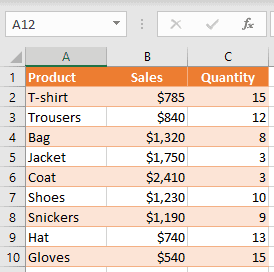
For creating a chart, I will be using the below data gear up, which contains products in column A, Sales value in column B, and Quantity value in cavalcade C.
In guild to create a chart, you lot need to follow the beneath steps:
- Select a range of values that you want to present on a chart (in this example B1:C10)
- Go to the Insert tab
- Select Insert Scatter chart icon
- Cull the Scatter nautical chart
As a issue, yous go the scatter chart as shown below (where I accept highlighted the axis using the arrow).
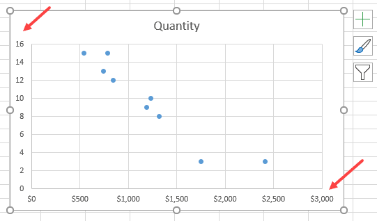
This nautical chart has the Ten-axis (horizontal) with values from the Sales column and Y-axis (vertical) with values from the Quantity column.
When y'all create a chart in Excel, it automatically decides the range that needs to be shown in the axis.
Now that's all skillful! Merely what if I want a chart where Sales is in Y-Centrality and Quantity in X-centrality.
Thankfully, Excel allows you to easily switch the Ten and Y axis with a few clicks.
Let'due south come across how to exercise this!
Switch X and Y Centrality in Excel
Now, if y'all want to display Sales values on the Y-axis and Quantity values on Ten-centrality, you need to switch the axis in the chart.
Below are the steps to do this:
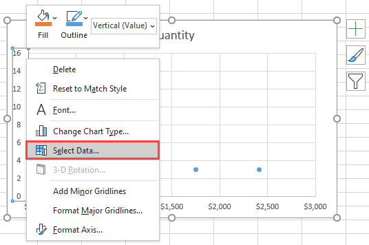
- Yous need to right-click on one of the axes and choose Select Data. This way you lot can besides alter the data source for the nautical chart.
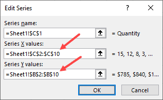
- In the 'Select Data Source' dialog box, you can see vertical values (Series), which is 10 axis (Quantity). As well, on the right side there are horizontal values (Category), which is Y axis (Sales). You have to click on the Edit on the left side in order to switch axes.
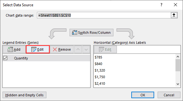
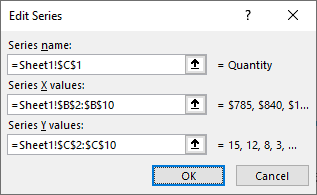
- In the pop upwards window, y'all can see that Series 10 values are range "=Sheet1!$B$2:$B$10", and the Series Y values are range "=Sheet1!$C$2:$C$ten".
- In order to switch values, you have to swap these 2 ranges, so that the range for serial Ten becomes a range for series Y and vice versa. So, in Series Ten values, enter "=Sheet1!$C$2:$C$10", and in Serial Y values, enter "=Sheet1!$B$2:$B$10".
- After you confirm changes, you lot will be redirected back to the Select Information Source window, and click OK.
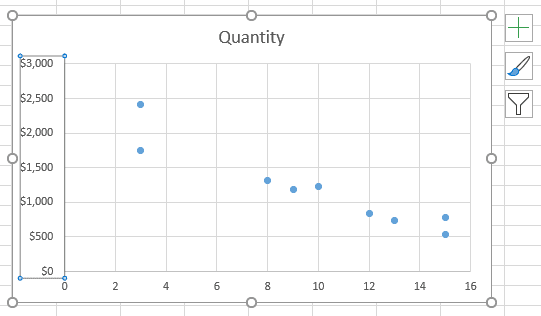
Finally, your chart has a switched axis. As yous can see, Sales values are now on the Y-axis, and Quantity values are on the X-axis.
Rearrange the Information to Specify the Axis
The above method works great when you lot have already created the nautical chart and you lot want to bandy the centrality.
But if you haven't created the nautical chart already, one way could be to rearrange the data and then that Excel picks up the information and plots information technology on the X and Y centrality every bit per your needs.
Excel by default sets the offset column of the data source on the X-axis, and the 2nd cavalcade on the Y-axis.
In this instance, you can only motility Quantity in column B, and Sales in cavalcade C.
Switching the axis option in a chart gives you more flexibility for adjusting the chart axis. Also, this way you don't need to change any data in your sheet.
So these are ii elementary and easy ways to switch the axis in Excel charts.
While I have shown an example of a besprinkle chart in this tutorial, you lot tin employ the same steps to switch axis in example of any chart in Excel.
I hope you lot found this Excel tutorial useful!
Other Excel tutorials you may also like:
- How to Move a Chart to a New Canvas in Excel
- How to Insert an Excel file into MS Word (3 Like shooting fish in a barrel Ways)
- How to Create Bar of Pie Chart in Excel?
- How to Insert Chart Title in Excel?

Source: https://spreadsheetplanet.com/switch-axis-in-excel/
Posted by: taylortheard.blogspot.com
0 Response to "How To Change X Axis Range In Excel"
Post a Comment